A version of this article first appeared in the December 2019 edition of our free newsletter, to subscribe click here

Authors note: In this installment, mesh density – or the art of being just conservative enough we touch on the differences between FE modeling composite and metal structures. first installment , second installment.

In this ‘chapter’ we will cover the issue of mesh density and how we decide the mesh densities for the finite element models we create.

Let’s start with some obvious basics and some general problems and advantages of finite element modelling versus hand analysis.

Finite element modeling is different to hand analysis in two key ways (assuming you stick to linear static solutions which we try to do as often as we can).

1. A finite element model automatically resolves static indeterminacy created by considering the stiffness of the structure. It does not make any assumptions (other than the assumptions you build into the model) on where the load is going to go.
2. A finite element model takes account of all modeled geometry and this generates Kt effects within the model results.

The inclusion of Kt effects in the model output has a conservative effect on model results used for static analysis of metal structures. For metal structure static analysis, Kt effects generally should not be considered. Once you get to higher mesh densities in finite element models of metal structure, it is unavoidable to lump in Kt effects with the results, and you have to either live with the conservatism or you can try to isolate the field stress without the Kt effect.

There is a general misunderstanding of this issue. As finite element models of metal structure become more detailed and ‘representative’, they invariably include greater geometric stress concentration effects. This, along with a conservative interpretation of 25.305(a), has driven unnecessary weight into metal aircraft structure for the last 10 years or more.

Kt effects in finite element models of metal structure can be mitigated by extracting the local loads and moments and performing a hand analysis of the region. You use the model stress results directly and try to calculate the local Kt effect using a standard reference (Peterson) and divide the model stress by that factor (not recommended) or use a strain energy conversion method such as the Neuber method.

In the end, for metal, it is quicker and easier to use a lower density mesh that avoids Kt effects, extract the local loads and use them for a classical hand analysis. If you are interested in local detailed behavior, plasticity and fatigue/damage tolerance, a supplemental local fine mesh model is the way to go.

Composites are different.

Well, we know that. To be specific, the fundamental behavior of composites combined with the way in which we qualify composite primary structure give us a different set of drivers for how we create a finite element model.

Composites, at the scale we are interested in, do not display plastic behavior. Therefore, a linear static model should accurately predict failure for composite structure because there is no plastic redistribution.

Because there is no plastic behavior or plastic load redistribution, Kt’s do matter. Kt’s will influence the static failure of composite structure.

With composite primary structure, it is not that simple. For aircraft primary structure we are compelled to acknowledge damage tolerance. The most practical way to deal with damage growth in composite structure is to ensure it does not happen. As outlined in section 4.1.6 of our free textbook, laminate strain is limited to a value at ultimate level (defined by CAI testing and open hole testing of panels). When structure is sized at ultimate level using these strain values, damage will not grow from those same features (impact damage and open holes) at service level loads and strain.

The allowable laminate strain we use has a level of Kt included. For an open hole, that level of Kt is at least 3.0, and in the case of compression after impact it is greater than 4.0.

These allowable strain values presuppose that the laminate has the potential for manufacturing flaws; porosity, voids, inclusion, etc., up to a Kt 4.0 and provides mitigation for these flaws.

People are generally concerned that we do take account of Kt’s in composite finite element models. However, if we create a fine mesh model of a panel with a circular hole, the strain results from the model at the critical area at the hole edge will include a Kt of over 3.0. If we then use a CAI strain allowable to size the laminate, the local Kt effect we are accounting for is the combination of the Kt from the mesh and the Kt built into the allowable strain value. The Kt value you will account for will be over 12.0. This is clearly too conservative.

So, in a perfect world you could take the same approach as when you create a metal finite element model. You could use a relatively low mesh density and ignore features that generate Kt’s less than 3 or 4. This means you rely on the Kt built into the allowable strain value to cover you for the Kt generated by geometry in the structure. In this case you only have to worry about very poor geometry (which should always be avoided).

If we only used our composite large scale finite element models for linear static analysis the story would end here.

However……

There are few satisfactory hand buckling analysis methods for composites. We have complied some in our textbook, section 16.2, but I prefer to use the finite element model for a composite buckling solution. For buckling of metal structures, I.am happy using either finite element model or hand analysis, as we usually get good correlation between the two.

So our composite finite element models have to do double duty, and they serve as our general strain prediction tool. We also use them to predict the onset of buckling. And, the model mesh density has to be at a resolution that will give good buckling results.

In order to accurately predict the onset of buckling we need to include geometric features that could affect the onset of buckling. Holes, cutouts, etc. So there is some unavoidable double dipping caused by the combination of Geometric Kt from the structure and the Kt built into the allowable strain value.

The mesh has to be a reasonable density for credible buckling analysis. For larger scale models we will usually keep to a nodal pitch of between 1 inches (2.54 cm) and 2 inches (5.08 cm).

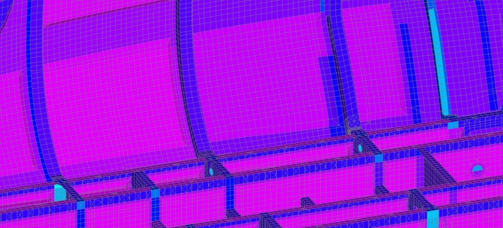
Example of fuselage finite element model. Fuselage side wall, cored composite and frames, approx 1.0in element size. This mesh was created by Nirav Shukla – who is about the best engineer I have worked with at creating nicely ordered finite element meshes.

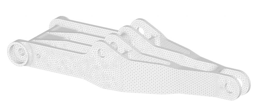
For detail models we just try to keep the nodes and elements to a reasonable number, so we can run the model quickly for a range of solutions and the data it produces does not take up too much space. I usually start to think the mesh is too dense or the model too detailed if we exceed 500,000 nodes. Generally we try to keep the number of nodes as low as practical to make hand stitching of the mesh, data management and other issues easier.

Some example meshes:

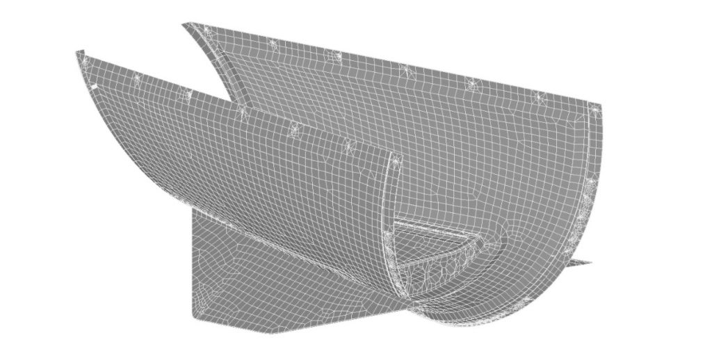
‘Quick’ cored composite tail fairing with ventral stakes. This has a general node pitch of 0.75in and has around 10,000 nodes. Note the ‘messy’ meshing regions around the attachment holes at the edge of the fairing. Where the auto-mesher creates an irregular mesh in a non-critical region we do not always correct. For this example we know the attachment loads would be low, so we let these poorly meshed regions stay. We used this model for static strain prediction only.

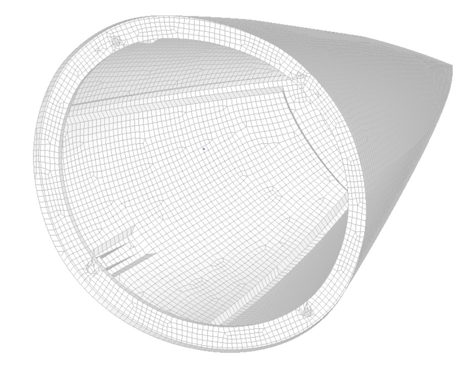
Cored composite model of replacement radome for fighter aircraft. (see later article in this newsletter) This has a general node pitch of 0.5in and a total of around 16,000 nodes. We used this model for static strain prediction and linear buckling checks (see next article).

No matter the mesh density you use, you should not automatically trust the results produced by finite element model. A finer, more detailed model will be more impressive to look at but can be wrong in many more subtle and complex ways than a simple model.

It is important to bear in mind that all models are ‘wrong’, in that they cannot perfectly emulate the real world. Make sure you understand the extent of the error to the best of your ability and the tools available.

It is often better to settle for a simple model with limitations that are understood, than a more impressive complex model with many more known and unknown inaccuracies.