A version of this article first appeared in the February 2020 edition of our free newsletter, to subscribe click here
We return to composite (and other structure) finite element modelling and tackle joints in this issue. To state the obvious joints are where different pieces of structure are joined to each other.
For most joint modelling we are interested in extracting the loads from the model at the joint interface and carrying out an external calculation to give a margin of safety.
This is because the behaviour of joint is more complex than the general structure and a finite element model requires a high degree of complexity to represent all of the aspects and features of a joint (bonded or mechanically fastened). It is much more efficient to make the stiffness of the area of the joint broadly representative and design the mesh to make it easy to extract the local loads.
At least that’s the correct approach for larger scale models. For smaller scale models I have seen ( and created) detailed models of mechanical fasteners and adhesive bond lines. But whatever those more detailed models tell me I always end up relying on extracting the loads and running a hand check to make sure the joint will be good.
Adhesively bonded joints:
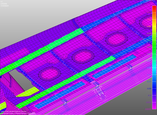
For adhesively bonded joints in large scale models we will model the flange that is bonded into the skin mesh. This is done to better model the stiffness of the vonded joint interface. This also helps with the local stiffness of this region for the buckling solution
We have found that if the core ends in the correct position and the bonded flange against the skin is not modelled you can start to get compression buckles of the stretch of uncored skin. This is because the bonded flange creates additional out of plane bending stiffness that stops the compression buckle in these regions.
The element loads form the rib (or frame) web can ex extracted and used to check the bondline for shear transfer and peel in the following way.
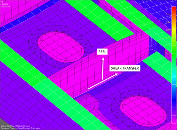
This is the simplest and most robust way we have found to deal with adhesive bonds at a large scale.
For detailed models we will sometimes model the adhesive as solid elements, this is the finite element model for the edge of transparency:
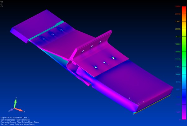
One of these interfaces uses a bonded joint, in this case we modelled the joint as a set of solid elements that share the nodes of the laminate elements either side of the joint. This does not help us determine if the bond is likely to fail, but it is a more accurate representation of the stiffness of the intact bondline.
The von mises stress in the solid elements representing the bondline looks like this:
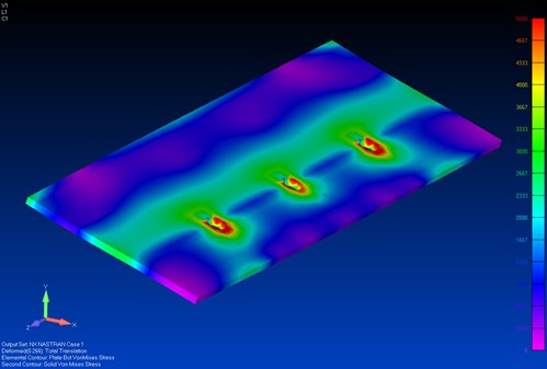
This indicates there is a peak von mises stress of around 5,000psi. In general we use 1,000psi as the average bond shear ultimate allowable.
And we generally assume 200lb/in ultimate bond peel allowable.
Interpreting whether the bond line would fail is not simple given the above results. How do these results translate to our 1,000psi average shear stress allowable? This test article carried 1.5 times the load applied to the finite element model without failing this bondline.
We also went in to pass the ultimate pressure load for the fuselage with this design of windshield installation.
So we ignored the results from the elements that modelled the adhesive, but it gave the local region the correct stiffness for the resolution of results we required from the laminate.
Mechanical Joints
In general differentiate between rivets and bolts. We treat rivets like bondlines – we model them as a continuous connection at the nodes and extract the load flows from the local elements and calculate the peak load on the rivets.
For bolts at major structural interfaces we generally mode the bolts as CBUSH elements.
We center a node in the fastener hole of the fitting using a REB2 elements.
We create a mating node at the position of the hole in the mating item.
We connect the two nodes with a CBUSH Spring/Damper Element.
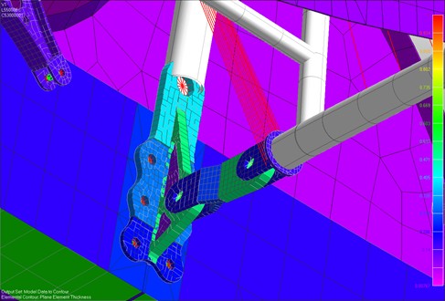
A typical fitting to wing spar is shown below:
We use a fictional set of stiffnesses for the CBUSH element:
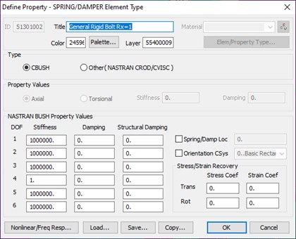
We do not leave any of the stiffnesses as zero. This is a trick to avoid unrestrained degrees of freedom. Of course you check the deflection of the model and if the deflection is excessive this may be down to a spring element degree of freedom allowing the model to run but also allowing very large deflections……
So we force the theoretical bolt to transfer tension, shear and bending (but not torsion) as if it were infinitely stiff.
We do not take account of the local theoretical fastener spring stiffness. This is because the stiffness is partly provided by the local stiffness of the interfacing items, in this case the wing fitting and the rear spar web. If we account for these in the fastener stiffness there is some element of double accounting.
This approach is easier and likely just as inaccurate.
As we do not model material plasticity it this scale of the model we are not taking account of load redistribution at the point of bearing yield so the linear model is not representative so the level of accuracy is further degraded for ultimate level loads.
For all of the joints we have sized using this approach we have seen no failures on test of the fasteners at the interface or the interface components at the fastener locations.
We do have to think about the moments carried by the elements representing the fasteners though. There is a method for doing this, this is defined in section 12.2.8 of our structures textbook:
The analysis spreadsheet is here: https://www.abbottaerospace.com/downloads/aa-sm-027-005/
In this method you can override the ‘M’ value with the resulting moment from the CBUSH element results and set the ‘P’ as the tension load. ‘B’ should be the distance from the center of the hole to the edge of fitting. This will give you the effective total tension carried by the fastener.
We use this method of modelling fasteners for all resolution of models. I have been involved in projects where the fasteners are modelled using higher order methods (non linear gap elements, solid models with contact surfaces) but I am not convinced that they add a greater degree of accuracy when all the variables of a real life fastener installation and joint behaviour is considered.
What is your experience with the FE modelling of joints? We would love to hear from you.
Comment On This Post